change cell background color in excel by equal formulas

In this article, I will show you how to change cell background color automatically in excel with Conditional Formatting tool.

Conditional formatting: Easily spot trends and patterns in your data using bars, color, and icons to visually highlight important values.

When working in Excel, have you ever faced with complicated and sometimes repeated data? A few redundant data will affect the entire calculation result so you need to find and remove them.

How to change cell background color automatically in excel by equal formulas?

Step 1: Click on the value box you need to color, press Ctrl + A if you want to select all the data => then click on Conditional Formatting => select New Rules.

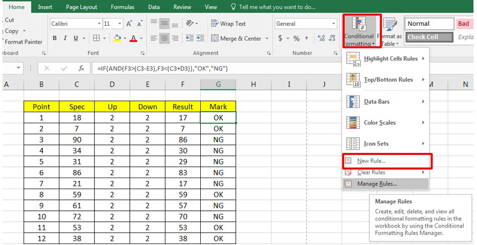
Step 2: In the  new formatting rule dialog box,  in the select a rule type, select Format only cells that contain to format the cell according to its value. Select cell value and equal at format only cells with. 
For example, at step one you choose NG to create the background color, here you enter NG.

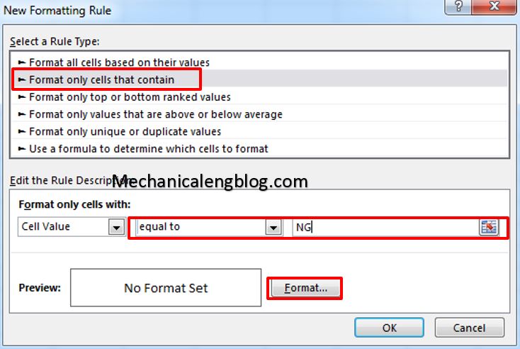
Next, click Format => Format Cells dialog box appears, click Tab Fill, and choose the color tone you want to fill in the content box. At this tutorial, I select red color, then click OK.

Step 3: After color formatting NG text is completed, in the dialog box Conditional Formatting Rules Manager, click Apply => and OK to save the result and exit the dialog box.

From now on, when you enter the characters like NG, Excel will automatically color them. The sequence is performed similarly to other data regions.

Conclusion.
Using the Conditional Formatting tool, you can similarly color with many repeatable values to easily distinguish them during your work. Also makes it easier for you to control what you enter and what data is on your Excel spreadsheets. Hopefully with today’s small tips will be helpful to you. Good luck!